
Contents
- The table every example runs on
- Every function by family
- What the grid handles besides functions
- What is deliberately missing
Type one and watch it resolve
The first formula exercise is open without an account and runs in the same grid these examples were produced in.
Excel functions list, with a worked example for every one
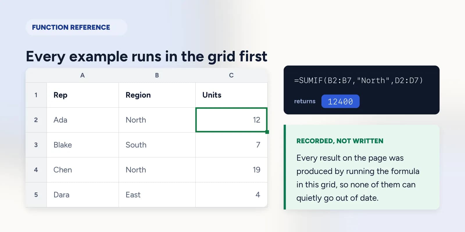
All 84 functions, grouped by the job they do, with Excel's own argument names and a formula you can copy. Every result below was produced by running the formula in the spreadsheet on this site, not typed in by hand, so none of them can quietly go out of date.

The table every example runs on
Rather than invent a different set of cells for every entry, every example that needs data is written against this one table. Column C has a gap on purpose: it is what makes COUNT and COUNTA disagree about the same column, and it is why AVERAGE divides by five rather than six.
| Row | A | B | C | D | E | F |
|---|---|---|---|---|---|---|
| 1 | Rep | Region | Units | Revenue | Joined | Grade |
| 2 | Ada | North | 12 | 4800 | 15 Jan 2024 | A |
| 3 | Blake | South | 7 | 2100 | 2 Mar 2024 | C |
| 4 | Chen | North | 19 | 7600 | 20 Nov 2023 | A |
| 5 | Dara | East | 4 | 1200 | 8 Jun 2024 | B |
| 6 | Eli | South | 15 | 5250 | 30 Sep 2023 | B |
| 7 | Fay | East | — | 900 | 11 Feb 2024 | C |
Joined holds real dates, built with DATE(), because a spreadsheet stores a date as a count of days and will not read one out of a typed-in string. That is also why one date minus another gives you a number of days.
Every function by family
Square brackets in a syntax line mark an optional argument. The practise link on 41 of them opens an exercise whose answer uses that function, marked on the formula you write rather than on the number you arrive at.
Maths and statistics
Totals, averages and the spread around them. These are the functions a spreadsheet is mostly made of, and the ones whose edge cases, blanks, zeros and text sitting in a number column, cause the most quietly wrong answers.
SUM
practiseAdds up numbers and ranges.
A blank cell inside the range is skipped, not read as a zero.
=SUM(C2:C7)returns57AVERAGE
practiseThe mean of the numbers, ignoring text and blanks.
Divides by five, not six: the blank in C7 is not an entry. A zero would have been.
=AVERAGE(C2:C7)returns11.4COUNT
practiseHow many cells hold a number.
The heading in C1 is text, so COUNT ignores it. Useful as a free check on a column you do not trust.
=COUNT(C1:C7)returns5COUNTA
practiseHow many cells are not empty.
Counts anything that is not empty, heading included. The gap between this and COUNT is how many cells hold something that is not a number.
=COUNTA(C1:C7)returns6COUNTBLANK
How many cells in a range are empty.
=COUNTBLANK(C2:C7)returns1MIN
practiseThe smallest number.
=MIN(C2:C7)returns4MAX
practiseThe largest number.
=MAX(C2:C7)returns19MEDIAN
practiseThe middle value once the numbers are in order.
The middle value rather than the mean, which is what to reach for when one enormous row is dragging an average around.
=MEDIAN(C2:C7)returns12MODE.SNGL
The most frequent number.
=MODE.SNGL(4, 7, 7, 12)returns7STDEV.S
practiseSpread of a sample.
For a sample, which is nearly always what a spreadsheet column is.
=ROUND(STDEV.S(C2:C7), 2)returns6.02STDEV.P
Spread of a whole population.
For a whole population. Use it only when the rows really are everybody.
=ROUND(STDEV.P(C2:C7), 2)returns5.39VAR.S
Variance of a sample.
=VAR.S(C2:C7)returns36.3QUARTILE.INC
practiseThe value a quarter of the way through the data.
=QUARTILE.INC(C2:C7, 1)returns7PERCENTILE.INC
The value at a given percentile.
=PERCENTILE.INC(C2:C7, 0.9)returns17.4LARGE
practiseThe nth largest number.
The second largest. LARGE with k of 1 is MAX.
=LARGE(C2:C7, 2)returns15SMALL
The nth smallest number.
=SMALL(C2:C7, 2)returns7CORREL
practiseHow strongly two columns move together, from -1 to 1.
Near 1 means the two columns rise together. It is not evidence that one causes the other.
=ROUND(CORREL(C2:C6, D2:D6), 2)returns0.99SUMPRODUCT
practiseMultiplies ranges row by row, then adds the results.
Multiplies each row's pair and totals the lot, which is how a weighted average gets its numerator.
=SUMPRODUCT(C2:C6, D2:D6)returns300250PRODUCT
Multiplies numbers together.
=PRODUCT(4, 5, 3)returns60ROUND
practiseRounds to a number of decimal places.
=ROUND(3.14159, 2)returns3.14ROUNDUP
Rounds away from zero.
Away from zero, so −4.21 rounds up to −4.3.
=ROUNDUP(4.21, 1)returns4.3ROUNDDOWN
Rounds towards zero.
=ROUNDDOWN(4.29, 1)returns4.2ABS
Strips the minus sign.
=ABS(-250)returns250SQRT
Square root.
=SQRT(144)returns12POWER
Raises a number to a power.
=POWER(2, 10)returns1024INT
Rounds down to a whole number.
Always downwards, so INT of −7.9 is −8, not −7.
=INT(7.9)returns7MOD
The remainder after a division.
The remainder. MOD(row, 2) is the usual way to ask whether a row is odd or even.
=MOD(17, 5)returns2RANK.EQ
practiseWhere a number sits in a list.
Largest first by default. Add a third argument of 1 to rank smallest first.
=RANK.EQ(C2, C2:C7)returns3
Logic and error handling
Asking a question of a row and acting on the answer, and catching the errors that follow. The syntax is never the hard part here. The boundary is: whether a test uses > or >=, and which test comes first.
IF
practisePicks one of two answers based on a test.
=IF(C2>10, "Target met", "Below")returnsTarget metIFS
practiseTests several conditions in order and returns the first match.
Stops at the first test that passes, so the order of the tests is the whole formula. A final TRUE acts as the catch-all.
=IFS(C5>=15, "High", C5>=8, "Mid", TRUE, "Low")returnsLowAND
practiseTrue only when everything is true.
=AND(C2>10, B2="North")returnsTRUEOR
practiseTrue when at least one thing is true.
=OR(C5>10, B5="East")returnsTRUENOT
Flips true and false.
=NOT(C5>10)returnsTRUEXOR
True when an odd number of the tests are true.
True when an odd number of the tests pass, which for two tests means exactly one of them.
=XOR(C2>10, C5>10)returnsTRUETRUE
The value TRUE.
A value, not a function call: written bare, with no brackets.
=TRUEreturnsTRUEFALSE
The value FALSE.
=FALSEreturnsFALSEIFERROR
practiseReplaces an error with something readable.
Catches every error, which is also the risk: it will hide a genuine #REF! as readily as the #N/A you meant to tidy.
=IFERROR(D2/0, "No figure")returnsNo figureIFNA
Replaces #N/A only.
Catches only #N/A, so a broken reference still shows up as broken. Safer than IFERROR around a lookup.
=IFNA(VLOOKUP("Gus", A2:D7, 4, FALSE), "Not on the list")returnsNot on the listISERROR
True when the value is any error.
=ISERROR(D2/0)returnsTRUEISNA
True when the value is #N/A.
=ISNA(MATCH("Gus", A2:A7, 0))returnsTRUEISBLANK
True when the cell is empty.
True only for a genuinely empty cell. A cell holding "" looks empty and is not.
=ISBLANK(C7)returnsTRUEISNUMBER
True when the cell really holds a number.
The quickest answer to why won't this column add up: run it down the column and look for FALSE.
=ISNUMBER(C2)returnsTRUEISTEXT
True when the cell holds text.
=ISTEXT(A2)returnsTRUE
Conditional counts and totals
Count, add or average only the rows that match. The criteria argument is the part that looks wrong the first time: a comparison goes inside quotes, ">10", because the operator and the number are handed over together.
COUNTIF
practiseCounts the cells that meet one condition.
=COUNTIF(B2:B7, "North")returns2COUNTIFS
practiseCounts the cells that meet every condition.
Every condition has to hold on the same row. The ranges must be the same shape.
=COUNTIFS(B2:B7, "South", C2:C7, ">10")returns1SUMIF
practiseAdds up only the cells that meet a condition.
The range tested and the range added are different arguments, which is the argument order people get wrong.
=SUMIF(B2:B7, "North", D2:D7)returns12400SUMIFS
practiseAdds up the cells that meet every condition.
Reverse of SUMIF: here the range being added comes first.
=SUMIFS(D2:D7, B2:B7, "East", C2:C7, ">3")returns1200AVERAGEIF
practiseAverages only the cells that meet a condition.
=AVERAGEIF(B2:B7, "South", D2:D7)returns3675AVERAGEIFS
Averages the cells that meet every condition.
=AVERAGEIFS(D2:D7, F2:F7, "A")returns6200MAXIFS
The largest value among the cells that match.
=MAXIFS(D2:D7, B2:B7, "North")returns7600MINIFS
The smallest value among the cells that match.
=MINIFS(D2:D7, B2:B7, "South")returns2100
Lookup and reference
Finding a row by something you know about it and reading a different column from it. This is where most spreadsheet work actually happens, and where XLOOKUP and INDEX with MATCH each fix something VLOOKUP cannot.
VLOOKUP
practiseFinds a row by its first column and reads across.
The last argument is not optional in practice. Leave it off and Excel looks for the nearest match, which on unsorted data returns a confidently wrong row.
=VLOOKUP("Chen", A2:D7, 4, FALSE)returns7600HLOOKUP
Finds a column by its first row and reads down.
VLOOKUP turned on its side, for a table laid out across rather than down.
=HLOOKUP("Revenue", A1:D7, 3, FALSE)returns2100XLOOKUP
practiseFinds a value in one range and returns the matching item from another.
Two separate ranges instead of a column number, so inserting a column cannot silently break it. Exact match is the default.
=XLOOKUP("Dara", A2:A7, D2:D7)returns1200INDEX
practiseReads the cell at a row and column position in a range.
Position in, value out. On its own it is rarely useful; with MATCH supplying the row number it replaces VLOOKUP.
=INDEX(A2:D7, 3, 1)returnsChenMATCH
practiseReturns the position of a value in a range.
The third argument of 0 means exact. Without it MATCH assumes the list is sorted.
=MATCH("Eli", A2:A7, 0)returns5CHOOSE
Picks the nth of the values that follow.
=CHOOSE(2, "Gold", "Silver", "Bronze")returnsSilverROWS
How many rows a range covers.
=ROWS(A2:D7)returns6COLUMNS
How many columns a range covers.
=COLUMNS(A1:F1)returns6
Text
Cutting, joining and cleaning text. Usually reached for because data arrived in one column that should have been two, or with spaces that stop a lookup matching anything.
LEN
practiseHow many characters, spaces included.
Spaces count, which is how a stray trailing space gets caught.
=LEN("Spreadsheet")returns11LEFT
practiseThe first few characters.
=LEFT("Spreadsheet", 6)returnsSpreadRIGHT
practiseThe last few characters.
=RIGHT("Spreadsheet", 5)returnssheetMID
practiseCharacters from the middle, by start position and length.
Counting starts at 1, not 0.
=MID("North-2024-Q1", 7, 4)returns2024TRIM
practiseRemoves stray spaces from both ends and collapses runs inside.
Both ends stripped and runs inside collapsed to one space. The usual fix for a lookup that matches nothing for no visible reason.
=TRIM(" North Star ")returnsNorth StarUPPER
ALL CAPITALS.
=UPPER("north")returnsNORTHLOWER
all lower case.
=LOWER("North")returnsnorthPROPER
practiseCapitalises The First Letter Of Each Word.
=PROPER("ada north")returnsAda NorthCONCAT
practiseJoins values into one piece of text.
The & operator does the same job in less space: A2 & " — " & B2.
=CONCAT(A2, " — ", B2)returnsAda — NorthCONCATENATE
Joins values into one piece of text.
The older name for CONCAT, kept because older workbooks are full of it.
=CONCATENATE(A2, " — ", B2)returnsAda — NorthTEXTJOIN
Joins values with a separator, optionally skipping blanks.
The one that takes a range, so a whole column becomes one comma-separated line.
=TEXTJOIN(", ", TRUE, A2:A4)returnsAda, Blake, ChenSUBSTITUTE
practiseReplaces every copy of one piece of text with another.
Matches on content. REPLACE matches on position.
=SUBSTITUTE("2024-Q1", "-", " ")returns2024 Q1REPLACE
Replaces characters by position.
=REPLACE("2024-Q1", 1, 4, "2025")returns2025-Q1FIND
practiseWhere one piece of text starts inside another. Case-sensitive.
Case-sensitive, and returns #VALUE! rather than 0 when the text is not there.
=FIND("Q", "2024-Q1")returns6SEARCH
practiseLike FIND, but ignores capitals and allows wildcards.
Ignores capitals and takes wildcards, which is why it is the safer default of the two.
=SEARCH("q", "2024-Q1")returns6VALUE
Turns text that looks like a number into a real number.
Turns a number stored as text into a real one, the repair for a column that will not total.
=VALUE("1200")returns1200REPT
Repeats text a number of times.
Makes an in-cell bar chart when fed a count.
=REPT("*", 5)returns*****EXACT
True only when two pieces of text match capital for capital.
The = operator ignores capitals. EXACT does not.
=EXACT("North", "north")returnsFALSETEXT
Formats a number as text.
Returns text, so the result can be joined to a sentence but can no longer be added up.
=TEXT(0.812, "0%")returns81%
Dates
A date in a spreadsheet is a number counting days, which is why one date minus another gives you days and why a date can be sorted and averaged like anything else.
DATE
Builds a date from a year, month and day.
The way to build a date from three numbers. Typing 02/03/2024 into a cell here leaves you with text.
=DATE(2024, 3, 2)returns2 Mar 2024YEAR
practiseThe year of a date.
=YEAR(E4)returns2023MONTH
practiseThe month of a date, 1 to 12.
A number from 1 to 12, not a month name. TEXT turns it into one.
=MONTH(E2)returns1DAY
practiseThe day of the month.
=DAY(E6)returns30WEEKDAY
The day of the week, 1 = Sunday.
1 is Sunday by default, which catches people out every time: a Monday comes back as 2.
=WEEKDAY(E2)returns2DAYS
How many days between two dates.
Plain subtraction, E5 − E2, gives the same number, because a date is a day count.
=DAYS(E5, E2)returns145
What the grid handles besides functions
Functions are only half of a formula language. The grid also handles operator precedence, brackets, percent literals, & for joining text, comparison operators, relative and absolute references including mixed forms like B$2, and Excel’s error values, #DIV/0!, #VALUE!, #N/A, #NAME?, #REF! and #NUM!. Each error has an exercise that causes it on purpose, because recognising one on sight is faster than looking it up.
What is deliberately missing
This is a practice grid, not an Excel emulator. There are no multiple sheets, no ribbon, no right-click menus, no inserting or deleting rows and columns, no whole-column references like B:B, and no saving files. The reasoning is that the thinking transfers and the menus do not: what a range is, how a reference shifts, why an average can mislead and when a chart lies are identical in every spreadsheet program ever made, while the location of Remove Duplicates changes between releases.
Excel’s own library runs past 500 functions once the engineering, financial and database families are counted. The 84 here are the ones ordinary spreadsheet work is built from, and the list is generated from the engine, so it can never promise a function that answers with #NAME?.
Common questions
How many functions does Excel have?
Excel ships with over 500, counting the engineering, financial and database families most people never open. The number that matters is far smaller: this page lists 84, which is the set that covers ordinary spreadsheet work, and every one of them runs in the grid here.
What is the difference between a formula and a function in Excel?
A formula is anything you type after an equals sign, including plain arithmetic such as =B2*1.2. A function is a named operation you call inside a formula, such as SUM or VLOOKUP. Every function appears inside a formula; not every formula contains a function.
What are the most used Excel functions?
SUM, AVERAGE, COUNT, IF, COUNTIF, SUMIF and VLOOKUP or XLOOKUP account for most real spreadsheet work. Learn those seven properly, with their edge cases, and you can read almost any workbook somebody hands you.
Why does my formula return #VALUE! or #N/A?
#VALUE! usually means a function was handed text where it needed a number, often a number stored as text. #N/A means a lookup found nothing, frequently because of a trailing space TRIM would remove, or because an exact-match argument was left off a VLOOKUP. Both have exercises in the course that cause them on purpose.
Do these functions work in Google Sheets?
Nearly all of them, with the same arguments in the same order. Google Sheets uses the older STDEV and MODE spellings alongside the newer STDEV.S and MODE.SNGL, and its date handling differs at the edges. The thinking transfers unchanged.
Can I try these functions without installing Excel?
Yes. The grid on this site is a real spreadsheet engine running in the browser, and every example on this page was produced by it. Type a formula into any exercise and it calculates exactly as it does here.
A function list is no use until you have typed one
Every function above runs in the same grid the exercises use. Start with the one most spreadsheets are built out of, or browse the full catalogue with each exercise’s access shown.
You might also like
- Excel shortcuts for beginners: the 12 that actually save timeThe twelve Excel keyboard shortcuts a beginner should learn first, what each is for, and a working spreadsheet to practise every one of them. Free, no account.
- The Excel paste values shortcut, and when you actually want itCtrl+Shift+V pastes values only, dropping the formula behind the number. What that means, when to use it, when it quietly breaks a report, and a grid to try it in.
- How to remove duplicates in Excel without deleting the wrong rowsData, then Remove Duplicates. What Excel counts as a duplicate, why trailing spaces defeat it, how to check before you delete, and a working grid to try it in.